Abstract
When two similar apartments end up selling for roughly the same amount, do their asking prices begin in the same place? Not always. Some agents repeatedly appear on the lower side of their peers, some on the higher side, and most do not have a clear direction. The especially striking result is how balanced the two sides are.
This is a retrospective look at completed sales, motivated by the question of lockpris. The Swedish Estate Agents Inspectorate (FMI) defines it as deliberately setting an asking price below the home’s assessed market value or the price the seller is prepared to accept. It describes patterns without naming or ranking any agent and without identifying any property or address.
1. Dataset overview
The source contains 116,055 historical sale records. 318 agent profiles available. The source records span from 2016. In total, 44,246 complete and plausible apartment sales were eligible for matching.
Peer comparisons were possible under 7 exact normalized area labels. 4 were large and diverse enough for the area comparison later in the post.
Datapoints used:
- Asking price: reconstructed by the collector by dividing the final price by one plus the displayed price-change fraction.
- Final price: used as a retrospective total-price matching condition.
- Apartment size: recorded in square metres; prices are compared per square metre and size is also matched with a symmetric 10% band.
- Rooms: matched exactly in the primary rule.
- Timing: based on the sale date rather than the listing date.
- Housing area: normalized exactly for the primary analysis. No fuzzy matching or unreviewed geographic merging is performed.
- Agent: profile URL, hashed and used only inside the calculation.
2. Methodology
Each apartment is compared with sales handled by other agents that have the same recorded area and room count, sold within ±120 days, and are within 10.0% for size and 10.0% for final price. A comparison needs at least 10 peer sales from at least 3 other agents, with safeguards against one agent dominating the peer group.
For focal sale i, let xᵢ = log(Aᵢ / Sᵢ), where Aᵢ is asking price and Sᵢ is apartment size. The score compares that asking price per square metre with the peer median and scales the difference by the peers’ robust spread:
A score below zero means the asking price was below its peer reference; a score above zero means it was above. The robust median absolute deviation (MAD) is used instead of ordinary standard deviation so a few extreme peer prices have less influence.
Worked example: from apartment to score
This hypothetical example illustrates the calculation; it is not an actual listing or agent result.
- A 2-room, 50 m² apartment has an asking price of SEK 4.5 million and a final price of SEK 5.0 million. Its asking price is therefore SEK 90,000 per m².
- Its peers have the same normalized area and room count, fall within ±10% for size and final price, sold within ±120 days, and were handled by other agents. The group must also pass the peer-count, agent-count, concentration, and variation gates.
- Suppose the median peer asking price is SEK 100,000 per m² and the robust log-price scale, calculated as 1.4826 × MAD, is 0.08.
-
The listing score is:
Worked score [log(90,000) − log(100,000)] / 0.08 = log(0.9) / 0.08 ≈ −1.32
The result means the asking price is 1.32 robust scale units below this listing’s peer reference. It does not mean 1.32% below, and it is not by itself a lockpris classification.
Figure 1
From apartment inputs to a peer-relative score
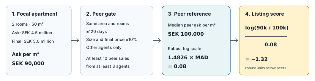
A hypothetical apartment passes through the peer-matching rules before its asking price per square metre is compared with the robust peer reference.
Note: The values are illustrative. No source listing, property, agent, address, or source row is represented.
Figure 2
The worked score on the peer-relative scale

The hypothetical score is 1.32 robust scale units below the peer reference.
Note: The score is not 1.32% lower and does not classify pricing conduct.
Each agent’s result is the median of their usable sale scores. An agent pattern is shown only with at least 30 usable sales across eight calendar quarters and comparisons involving at least five distinct peer agents. To check whether the pattern is stable over time, the analysis resamples observed calendar quarters while holding each sale’s observed peer reference fixed. These are conditional stability intervals: they measure variation over the observed periods and peers, not uncertainty from rebuilding every peer group.
One important limitation is built into the method. Final price occurs after the asking-price decision, and asking price is reconstructed from final price and the displayed price change. The comparison is therefore retrospective; final price is a matching condition, not an independent test of what happened before the sale.
3. How much could be compared?
The analysis starts with 44,246 eligible apartment sales. Only 11,301 found a peer group that passed every matching gate in the chosen rule. That is 25.5%, or about one sale in four.
Most excluded sales simply did not have ten sufficiently similar peer sales once area, rooms, time, size, and final price were considered together. That loss of coverage is deliberate: a smaller apples-to-apples sample is more useful for this question than a larger but looser comparison.
The time window illustrates the tradeoff. A shorter window stays closer to the local market moment but finds fewer matches; a wider window finds more matches but reaches farther across time. The chosen ±120-day rule is the middle ground. Other core changes to size and area matching are used as checks on the conclusion, not as competing headline results.
Figure 3
Usable comparisons increase with wider time windows
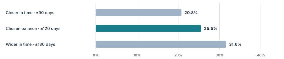
Of 44,246 eligible sales, 20.8% find a usable peer group within ±90 days, 25.5% within ±120 days, and 31.6% within ±180 days.
Note: The chosen ±120-day rule balances additional matches against reaching farther across time.
4. What stood out
In the main analysis, 114 agents had enough evidence to be summarized. The quarter-based stability range stayed below the peer benchmark for 25 agents, above it for 23, and crossed it for 66.
The mirror result became even clearer under the core matching checks. Among the 103 agents who qualified under every core check, 16 remained below and 16 remained above. Persistent higher scores are less consistent with repeatedly choosing a low starting price. Persistent lower scores are compatible with that pattern—but neither side proves or rules out lockpris on an individual sale.
Figure 4
Persistent patterns under every core check

Among 103 agents with enough evidence under every core matching check, 16 remained below, 71 were not one-sided, and 16 remained above.
Note: Direction alone is not a verdict about pricing conduct. No individual agent or sale is shown.
5. Did the areas look different?
The comparison includes 4 areas: Kungsholmen, Södermalm, Vasastan, and Östermalm. Together they cover 11,207 usable scores. Their median scores range from -0.014 to 0.037, very close to the peer benchmark of zero. The share of scores below zero ranges from 48.4% to 50.9%—roughly half in every group.
Figure 5
Area-relative scores remain close to balanced

The four qualifying areas cover 11,207 usable scores, with shares below the peer reference ranging from 48.4% to 50.9%.
Note: These are within-area comparisons, not absolute price comparisons or a formal test of an area effect.
These are area-relative scores: every apartment is already compared with peers inside the same recorded area. The area view therefore checks whether the resulting score distributions look different; it is not an absolute price comparison or a formal test of an area effect. The displayed names are readable versions of the exact normalized source labels; no broader geographic hierarchy is inferred.
6. Takeaway
The fun result is not that one pricing direction dominates. It is the symmetry: some selected agents repeatedly sit below their peers, an equally sized persistent group sits above them, and most do not stay clearly on either side. The 4 qualifying areas also look remarkably similar.
That does not establish intent, causation, responsibility, or a market-wide lockpris pattern. The source roster is selected rather than a census; asking price is reconstructed; final price is a post-listing matching condition; sale date is only a proxy for listing time; and condition, renovation, view, micro-location, seller circumstances, and marketing are not observed. The finding is a reason to look more closely, not a verdict.