This experiment has been run on an NVIDIA GeForce GTX 970 but shouldn’t have any problem using CPU only.
Feedforward and recurrent neural networks
Feedforward neural networks can approximate any continuous function, but only in the interval with enough training data density (Universal approximation theorem). Unlike feedforward neural networks, RNNs can use their internal states (memory) to store information from the input and the histories.
Method: The dataset is two different sine waves multiplied together to create the wave we want to predict. We train two models, a Feedforward neural network and an RNN, on this dataset. We send the predicted values back to the model to follow if the model has learned the function.
Hypothesis: Feedforward neural networks accuracy is expected to go down for every period, while RNN would remember.
import numpy as np
from matplotlib import pyplot as plt
from matplotlib.ticker import MaxNLocator
from DeepLearningModels import ModelFullyConnected, ModelRNN, sine_wave
Generate the signal
wave_1 = sine_wave(nsamples=50, periods=1, repeat=2)
wave_2 = sine_wave(nsamples=50, periods=2, repeat=2)
data = wave_1*wave_2

plt.title('Sine-wave \nOne period=50 sample, repeat=2')
plt.plot(data)
plt.show()
Figure 1
Wave used to train and test the models
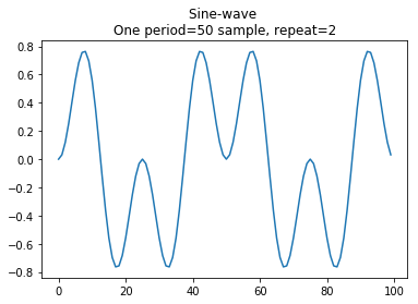
The combined wave repeats a changing sequence of positive and negative peaks, giving the models a periodic pattern to learn.
Create features and targets
time_back = 10
time_forward = time_back
batch_size = 1

dataX, dataY = [], []
for i in range(len(data)-time_back-time_forward):
    dataX.append(data[i:i+time_back])
    dataY.append(data[i+time_back:i+time_back+time_forward])
dataX = np.array(dataX)
dataY = np.array(dataY)

ax = plt.figure().gca()

ax.plot(range(time_forward), dataX[0], 'bo', label='dataX')
ax.plot(range(time_forward, 2*time_forward), dataY[0], 'ro', label='Predict')

ax.xaxis.set_major_locator(MaxNLocator(5, integer=True))
plt.legend()
plt.grid(axis='x')
Figure 2
Example input and prediction target
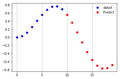
Each training example gives the model 10 consecutive values and asks it to predict the following 10 values.
dataX = dataX.reshape(len(dataX), batch_size, time_back)
print('dataX:', dataX.shape,'\ndataY:', dataY.shape, sep='')
dataX:(80, 1, 10)
dataY:(80, 10)
Create the models
fc_model = ModelFullyConnected(batch_size, dataX.shape, dataY.shape)
rnn_model = ModelRNN(batch_size, dataX.shape, dataY.shape)
Fully connected neural network
fc_model.create_model(nr_layers=3, units=30)
fc_model.fit(dataX, dataY)
fc_model.plot_training()
Figure 3
Fully connected model training history
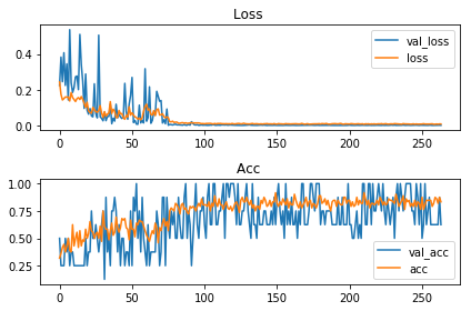
Training and validation loss fall toward zero, while the accuracy curves rise and remain variable over the recorded run.
Note: These are the notebook's training metrics, not an independent test result.
SimpleRNN
rnn_model.create_model(nr_layers=3, units=20)
rnn_model.fit(dataX, dataY)
rnn_model.plot_training()
Figure 4
SimpleRNN model training history
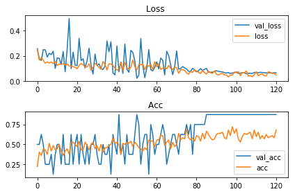
The recorded loss trends downward, while the accuracy curves rise with substantial variation during training.
Note: These are the notebook's training metrics, not an independent test result.
Compare the forecasts
plot_fc = fc_model.plot_predict(dataX[0:1], time_forward, len_range=100)
plot_rnn = rnn_model.plot_predict(dataX[0:1], time_forward, len_range=100)
plot_full = []
while len(plot_fc) > len(plot_full):
    plot_full.extend(data)

plt.figure(figsize=(10, 7))

plt.subplot(211)
plt.title(fc_model.model_information())
plt.plot(plot_full[time_forward:len(plot_fc)], 'r--')
plt.plot(plot_fc[:-time_forward], 'b')

plt.subplot(212)
plt.title(rnn_model.model_information())
plt.plot(plot_full[time_forward:len(plot_fc)], 'r--')
plt.plot(plot_rnn[:-time_forward], 'b')

plt.tight_layout()
plt.show()
Figure 5
Forecasts beyond the training sequence
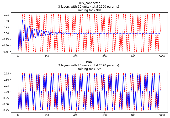
The fully connected model's forecast decays toward zero, whereas the RNN continues to track the amplitude and frequency of the reference wave.
Note: Predictions are fed back into each model to extend the forecast.
Conclusion: Feedforward neural networks are not great on data that have has a periodic quality. However, RNN can remember and have a “memory” about what they have “seen” before.
Discussion: When the Feedforward neural network model tries to predict the next value at zero, it has learned that the possibility is fifty-fifty. But the RNN model remembers the amplitude and frequency.